
Decoding the Encoder
The Secret Maps of Modern AI

AI's Hidden Language
I’ve been thinking a lot about a few topics that I would like to discuss that bridge technical AI concepts, but I worried that not everybody would be able to grasp them properly, and their implications might get lost in abstraction, and I find those implications to be the most important parts of the whole thing! For that reason I realized that maybe the best way to go forward would be to make a nice guide to some concepts that I find really integral in understanding how AI works. By the end, you’ll see how these maps reveal how machines—and perhaps humans—simplify reality.
We’ll start with everyday encoding, progress to neural networks, and finally uncover how encoders power systems like ChatGPT.
At the core of many AI systems lies a powerful tool called an encoder—a neural network component that compresses information into compact, meaningful representations. In this article, we’ll explore what encoders are, how they work, and why they’re integral to modern AI. By the end, you’ll understand how encoders create ‘maps’ of information that machines use to navigate complex tasks like language understanding and image recognition.
We’ll start with simple examples of encoding, progress to some core machine learning concepts, and conclude with how encoders fit into larger AI architectures.
Map and Territory?
When thinking about encoders, the first thing that comes to mind probably is something to do with ciphers, hidden meanings, weird symbols, or, who knows, the Enigma machine (I know at least that comes to my mind). However, encoding is a process we encounter in surprisingly simple forms. Let’s explore some familiar examples that demonstrate the power of encoding information.
Metro Maps: Simplifying complexity
Metro maps are a perfect illustration of encoding in action; we see them all the time around (at least if you live in a bigger city) without giving them much thought. These colorful diagrams transform the messy reality of a city’s geography into a clear, easily digestible format.

Consider the London Underground map: it distorts distances and shapes, simplifies complex routes into straight lines, uses color coding for different lines, and represents stations as simple dots. The encoding process takes quite a bit of artistic liberty as well to make the map easy to look at— it prioritizes clarity over geographic accuracy. The map preserves essential relationships and connections between stations and lines, while discarding unnecessary details like exact distances or street layout; but like this, you have no problem being able to tell in seconds where you are, where you are going, and from a few meters away in a crowded underground train nonetheless.
Morse code: Layered Encoding
Let’s take an interesting example that I’ve been thinking about recently: we all know about Morse code; each letter, symbol, and number corresponds to a certain string of dots and lines (short or long beeps). “Ok, Darius, so we have an encoding method. Cool. Now what?” So based on some restrictions of the system (the telegraph system), and to make things easier, like making sure it will work even with a poor signal, they went back to the most basic system of signaling—beeps, longer beeps, and no beeps. But it goes a bit beyond that; writing a whole text like that would take quite a long time, even for experienced operators, so they added another layer of encoding over that, and after a while they had their own dictionary of abbreviations that they use. Until recently, I just assumed (out of ignorance) that ok, they have some Ks-OK, BRBs-Be Right Back, or LOLs-Laughing Out Loud, but it goes way further than that, and I’ll show you an example of a Morse code transmission:
... ..--- -.-- --.. / -.. . / ... .---- .- -... -.-. / = --. .- / -.. .-. / --- -- / ..- .-. / .-. ... - / ..... -. -. / .... .-. / = --.- - .... / .- .-.. -- . .-. .. .- / --- .--. / .. ... / .--- --- .... -. / .... .-- ..--.. / ... ..--- -.-- --.. / -.. . / ... .---- .- -... -.-. / -.- -.
That directly translated to the English alphabet looks like this:
S2YZ DE S1ABC = GA DR OM UR RST 5NN HR = QTH ALMERIA = OP IS JOHN = HW? S2YZ DE S1ABC KN
Yeah, it still doesn’t really make any sense yet, so let’s translate that as well to plain English:
"To station S2YZ from S1ABC: Good afternoon, dear friend. Your signal report is 599 here. My location is Almeria. Operator is John. How do you copy? Over to you exclusively.”
And now we have something we can understand, mostly. Some of the substitutions are obvious: GA=Good Afternoon, UR=Your, HR=Here, or SOS, which we all know what it means, but not what it stands for too; but some are quite interesting, and they come with quite some history from Morse code users: DR OM = Dear Old Man, which is a term used for any male amateur radio operator; RST 5NN comes from Readability, Strength,Tone, which is a signal report format, and 5NN is 5 for excellent signal, N is a substitute for 9 because it is way shorter to write and means perfect readability, and another N for perfect tone.
So you take language, put it through an encoder (operator), it goes through a very restrictive medium, and with a decoder (another operator—we’ll talk about decoders later too), you have a clear message. Apparently the average speed is somewhere around 20-30 words per minute, with skilled operators going up to ~84 wpm, which is quite a bit faster than I can type on a keyboard!
Now that we’ve revised some encoding examples in familiar contexts, and shown how complex information can be simplified into more manageable forms, we should ask: What happens when the information we’re working with isn’t as straightforward as stations on a map, or dots and dashes?
Real-world data— whether it’s images, text, or sensor readings—is messy, high-dimensional, and full of nuance. To handle this complexity, we need tools that can do more than just simplify; they must also uncover hidden patterns and relationships that might be too obscure for us to identify. This is where neural networks come into play.
Neural networks are like the next level of encoding. Instead of human-designed rules (like Morse code abbreviations), they learn to create their own representations of data. These representations can capture intricate patterns that are impossible to define manually.
Just as Morse operators developed shorthand (73 = best regards), neural networks invent their own ‘dialects’ through training. But instead of human-devised abbreviations, they statistically derive patterns from data—a process we’ll now unpack.
Before we dive into encoders specifically, let’s take a quick detour to understand how neural networks work, why they’re so powerful, and how they set the stage for encoding in AI systems.
Neural Networks Demystified
To make sure I cover everything, I will do a quick run-through of some of the basics of neural networks.
Functions 101: The Atomic Unit
At its core, machine learning is about finding mathematical relationships, and that’s exactly what functions are! We all remember functions from middle school; all they do is show you the relationships between two (or more) variables. These can be whatever we want: apples and oranges (similar to middle school problems), house prices and square meters, height and weight, etc.
We’ll also use the Cartesian system to visualize those relationships more easily. Adding other variables, such as a and b (coefficient and bias, but the terms change a lot based on the field), in this case, lets us say more about the relationship, like scaling (how steep the line is) or adding constants (where the x=0 intersects with y) respectively. a could be by how much are oranges more expensive than apples, and b could be a flat tax you pay for importing them instead of growing them locally.

Using the Cartesian system and X and Y axes is just for convenience, as it's generally easier to visualize data like that. But as far as the concepts of functions and especially machine learning are concerned, you can do whatever you want. Leave X as numbers, drop the Y and use a “fishiness” scale to represent the relationships.

Although, in real life, is very rare to have such a straightforward relationship between only 2 variables.
Variables Go 3D: Enter the Matrix
Real-world data is rarely one-dimensional though, so let’s see what we can do about that. The answer is quite simple; just add another variable to the function equations:
Now we’re working in 3D space! Each input (x,y) gets transformed into z through weighted combinations (weighted as we have the extra 3,2 and 5 to model them as we want, basically representing how much each variable contributes to the output). Again, those can be whatever relationships you choose; X and Y for square meters of an apartment and distance from the downtown area respectively, and Z for the price of the apartment.

Or, if you prefer the “fishiness” scale, we can also continue with that:

This is the essence of what neural networks do—they combine multiple inputs with learned weights. Discussing how training or model learning works is quite a big topic as well, but a bit outside the purpose of this post, so we’ll leave that for another time. but in the meantime, you can use this analogy to get an idea about them: just as we learn from mistakes, neural networks adjust weights to minimize errors—a digital form of growth mindset if you will.
But this still is too simplistic for real-world data—relationships between variables often curve, bend, or twist in unexpected ways.
Real World Likes Curves
Nature usually doesn’t like straight lines that much, and that doesn’t exclude the math with which we try to describe nature with. Thankfully, math lets us put even more numbers around our Xs, not only coefficients, so we’ll have to move from linear functions to more complex ones like quadratic, cubic, or even more nonlinear ones.
Let’s start with a simple one, a quadratic function:
When we plot this, we get a curve—a parabola. This kind of non-linear relationship is common in real-world data: think of how temperature affects plant growth or how speed impacts fuel efficiency.

Here you can see how adding more terms affects the line, making it curvier and being able to describe stranger and stranger relationships; and these curves are just the beginning—that is how we are getting closer and closer to machine learning as well. We’ll basically stack a lot of those functions together and increase the complexity exponentially.
Changing Notations: ML Visualization
From here on, things are getting more and more complex, so to be able to understand them easier, in machine learning literature, we often represent these functions as neurons connected in layers. Each neuron performs a simple operation (like multiplying by a weight and adding a bias), and layers combine these operations into something much more powerful, but at their core, they are the same stuff—functions.
Let's take an example of a small network. Each connection represents a weight, and each neuron applies an activation function (like ReLU or sigmoid in general, but you can use whatever you want or whatever suits the case, like a quadratic activation function, although those are not as often used for reasons that have to do with the training procedure and how the math can become quite messy).

Here we have a 3-4-1 neural network. It has 3 inputs, then goes through a hidden layer (just terminology) of 4 neurons and outputs a single variable.
If we try to write this network’s formula, it would look like this:
Maybe it seems a bit daunting, but lets get through it step-by-step, in operational order (inner paranthesis first).
Hidden Layer Computation
Let’s try to decode this step by step to something we’re more used to:
Hidden Layer computation:
W₁: Weight matrix (4x3) connecting inputs to the hidden layer
Think of weights as dials controlling how much each input matters—like adjusting bass/treble on a stereo; but it “learns” how it sounds the best by adjusting them constantly and seeing how the new result is.
They are represented by all the white lines you see in the picture, connecting all inputs to all hidden layer neurons
x: Input vector (3x1)
The blue dots
b₁: Bias vector(3x1)
Biases are like a chef’s secret ingredient—always added, no matter the recipe.
Usually they are not depicted in ML graphs
σ: Activation function
depicted as the neurons
Think of them as filters that decide whether a neuron should 'fire' based on input strength. That’s where the “activation” term comes from.
This is the same as our multi-variable function z=3x+2y-5 from earlier but scaled up:
each neuron in the hidden layer computes its own “mini-function”, and instead of writing 4 formulas with 3 variables each, we will write them as a matrix of 4x3 (W₁), same for all the other variables as well.

This is how the matrices would look like as well.
for example, the first hidden neuron computes:
Just straight matrix multiplication, but with weirder symbols.
Output Layer Computation
W₂: Weight vector (1x4) connecting hidden layer to output
h: Hidden layer vector (4x1)
the one we just discussed earlier
b₂: Output bias (scalar)
This resembles the original linear function y=ax+b but now:
x is replaced by the hidden layer’s output h
the activation σ introduces non-linearity; it depends what activation function we choose to use, a lot of times it would be functions like sigmoids which squashes values between 0 and 1.
Why Activation Functions (σ) Matter
Without activation functions, neural networks would collapse into a single linear layer, so all the stacking and the neurons would just be a more or less useless complication. Having them will add the flexibility we would need, allowing networks to learn complex patterns instead of just straight lines.
Let’s look at an example:
without an activation function, the function we previously looked at would look like this:
which can be simplified to :

The Power of Complexity: Why Simple Models Aren't Enough
So now we have a better idea about neural networks, how they look, kinda what they do, but the question still remains: why? Why add all this complexity when we’ve seen that simple functions already can describe a lot of types of relationships?
The answer lies in the messiness of real-world data. Remember our “fishiness scale” example? In reality, determining whether something is a fish involves analyzing countless features; scales, fins, gills, habitat, movement patterns, and the relationships between these features are rarely straightforward. While our 3-variable example works in 3 dimensions, modern encoders operate in spaces with thousands of dimensions.
From Simple to Complex: The Power of Depth
Simple neural networks like our 3-4-1 example can learn basic patterns, but they quickly hit limitations. Think about trying to recognize handwritten digits—a seemingly simple task. A shallow network might struggle quite a bit with any deviation from perfect caligraphy. The same digit can be written in countless styles, slight variations in pen stroke might completely change what a simple model “sees”, or even background noise or smudges will confuse basic pattern recognition models.
This is where adding more layers (making networks "deeper") and more neurons (making networks "wider") transforms our humble neural network into something dramatically more powerful.
Each additional layer allows the network to learn progressively more abstract representations. Early layers might detect simple edges and contours, middle layers might recognize shapes and textures, while deeper layers identify complex objects and concepts. This hierarchical feature learning mirrors how our own visual system processes information as well!
Exponential Growth in Capabilities
When we add just a few more layers, the network's capabilities don't just increase linearly—they explode exponentially. Research shows that deep networks can achieve complexity that would require shallow networks to have an exponentially larger number of neurons to match. In other words, adding depth is a much more efficient way to increase modeling power than simply making layers wider.
For example, a 3-layer network might need millions of neurons in its middle layer to perform as well as a 10-layer network with just thousands of neurons per layer. This "depth efficiency" explains why modern AI models have grown from having thousands of parameters to billions while still being trainable with reasonable amounts of data.
The Surprising Efficiency of Complexity
The most counterintuitive aspect of complex neural networks is that despite having millions or billions of parameters (potential degrees of freedom), they don't require billions of training examples. This seeming paradox occurs because: Neural networks naturally find low-dimensional manifolds within their vast parameter space, they learn features gradually, with each layer constraining what the next layer can learn, and training techniques like batch normalization and residual connections (ResNets) help enforce correlation between layers, making learning more efficient.
This is similar to how proteins fold remarkably quickly despite having an astronomical number of possible configurations—the process follows an efficient path rather than randomly exploring all possibilities.
Still, this is also a double edge sword; as the complexity increses, the models also become harder and harder to interpret. Those potential degrees of freedom are exactly that, we can interpret all the parameters as a space with n-thousands dimensions, where each direction affects a certain aspect of the data we try to analyze.
Practical Necessity
For tasks like understanding language, recognizing faces, or interpreting medical images, simple models simply fall short. The patterns are too intricate, the variations too numerous, and the edge cases too important to ignore.
Complex models shine precisely where simple relationships break down—in the messy, nonlinear, interdependent world of real data. They can capture subtle patterns that simpler models miss entirely, making them indispensable for modern AI applications. But that’s exactly where encoders also come into play.
Bridging to Encoders: The AI Cartographers
We’ve explored how neural networks process data by combining inputs with weights and biases, passing them through activations functions, and stacking layers to extract complex patterns. But what if we wanted to do more than just process data? What if we wanted to summarize it, distill its essence, or map it into a simpler form while preserving its meaning? let's explore a specific architecture that leverages this complexity for a fascinating purpose: compression and representation learning.
This is where encoders come in. They’re like the cartographers of AI, creating simplified “maps” of data that machines can use to navigate complex problems. But instead of mapping cities or countries, encoders map concepts, patterns, and relationships. They are a bridge between the world of humans and the mathematical realm.
Intelligent Compression: The Essence of Encoding
Imagine you’re tasked with describing a painting over the phone. You can’t send the painting itself, so you have to summarize it. Describing Van Gogh’s Starry Night in 10 words would sounds something like: “Swirling blues, yellow stars, cypress tree, village below, emotional turbulence.”. And just like that you’ve encoded a 74MB image into 50 bytes; a 0.00007% of the original size!
The painting is the input data, your description is the encoded representation—a compact summary that captures the key elements, and the listener’s mental image is what happens when the encoded representation is reconstructed.
Encoders operate on those same principles: they take high-dimensional data (like an image with thousands of pixels) and compress it into a smaller representation that retains the most important features.
Autoencoders: The Mirror Architecture
To really understand encoders, let’s look at how we usually see them in the wild (literature): as an autoencoder. It combines two components: an encoder and a decoder.

Encoder: it takes the input data (e.g., an image or a sentence, or whatever you want to encode) and compresses it into a smaller version of itself. Like taking a 1920x1080 pixels image that might be reduced to only 32 numbers.
This process is highly dependent on the data, as the amount of compression certain data can handle differs. Imagine the difference between doing a very detailed description of a room with a minimalistic interior design, and a baroque one.
Bottleneck: this is where the latent space is. In here is the multi-dimensional space in which we try to encode our data; it’s like a compressed version of your data—a map where every point represents key features of the original input. The purpose of it is that it forces the network to prioritize what is most important about the input, and what are the most important details that it would need to keep in order to recreate the original input.
Decoder: Takes the compressed code and reconstructs the original input as closely as possible. This step ensure that the encoder captured meaningful information.
This set-up is also called an unsupervised model, as it only has the input data, and throught the training process, you force the network to find a space in which the data can be encoded, and keep as many details as possible. Most of the times this can be done, and shows us really interesting aspects of what we are analyzing. It would be like extracting all the important parts of a long text, without compromising on its meaning. Why use many words if less do trick (ok, maybe in some cases we’ll compromise on its artistic aspect).
Autoencoders in the Wild
To truly grasp the power of encoders, let’s explore how autoencoders work in real-world scenarios. Autoencoders are neural networks designed to compress data into a compact representation (latent space) and then reconstruct it. This process highlights their ability to distill complex information into its essence.
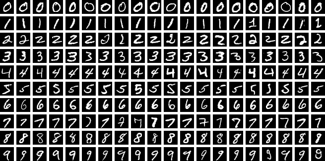
Let’s take one of the most known sandbox problems in Machine learning; the MNIST dataset. This dataset contains thousands of grayscale images of handwritten digits. Each image is 28x28 pixels, representing a high-dimensional space (784 dimensions). An autoencoder reduces this complexity by compressing each image into a latent space with far fewer dimensions—say, just 2 or 3.
Here’s how it works:
Encoding: The encoder transforms each 784-pixel image into a smaller vector (e.g., 3 numbers). This vector represents the most essential features of the digit.
Latent Space: These compressed vectors are clustered in latent space. For instance, all instances of the digit "7" might form a distinct cluster separate from "4."
Decoding: The decoder reconstructs the original image from its compressed representation, ensuring minimal loss of detail.

Latent Space: The Secret Language of AI
Latent space is where encoded data lives—a compressed representation that captures essential features while discarding noise and redundancy. Think of it as the "secret map" that AI uses to navigate information.
How Latent Space Works
When data is encoded into the latent space, high-dimensional input (like images or text) is reduced to a lower-dimensional form. The encoder prioritizes meaningful details, such as edges in an image or sentiment in text. Similar inputs are also grouped together, forming clusters that reveal hidden relationships (or more obvious ones, like how 7 could look like 1 based on personal handwritting styles).
Applications
Autoencoders are used in a lot of cases, I haven’t joked when I said they are the core of modern AI. Their application ranges from: denoising images, removing noise from images by learning clean representations in latent space, anomaly detection, by reconstructing normal patterns, deviations(anomalies) will stand out in the latent space, or generative tasks, with Variational autoencoders (VAEs), the latent space will be used to create new data by sampling from it, like searching where a “tree” is in the latent space and checking what is around it (usually other trees). I’ve also written before about some applications of VAEs as well if you are curious about a more in-depth view into how they would work.
The Practical Power: Why Encoders Matter
Encoders are everywhere in modern AI systems because they solve three key problems:
Pattern Recognition
Encoders learn to identify patterns automatically. For example: in images, they might detect edges, shapes, or specific objects like cats. In text, they might recognize grammar rules, emotional tones, or implied meanings.
Efficiency:
By compressing data into smaller representations, encoders make processing faster and more efficient. Imagine trying to send someone a whole book vs just sending its ISBN number. They both represent the same thing but in vastly different sizes.
Foundation for Advanced AI
Encoders are building blocks for systems like ChatGPT, Google Translate, image recognition systems, etc. They create compact representations of our world that these systems use to understand context and generate responses.
From Encoders to Monosemanticity
Here’s where things get even more fascinating: as encoders process data, most often they find quite obscure and abstract ways to represent it, but sometimes individual neurons can specialize in detecting specific feature of concepts. For example, a single neuron in an image encoder might light up only when there’s a cat in the frame, or, in most cases, edges, or basic shapes.
This phenomenon, where certain neurons respond exclusively to specific concepts is called monosemanticity, and it mirrors how our own brains work too! Just as your visual cortex has neurons dedicated to detecting edges or motion, AI encoders develop specialized “detectors”. We will explore this phenomenon exclusively in the next articles, as I find it profoundly interesting, and I believe it has a lot of relations with human cognition as well.
Beyond Encoders: Pathways to Monosemanticity
So let’s see what have we done so far. We looked a bit at the idea of encoding information and what it means. We speedran through neural networks and saw how at their core, they are just a bunch of stacked functions (although I’m quite reductionist with this statement, and I will delve deeper in the future into this; how even though mathematically reducible to function compositions, networks exhibit emergent behaviours unanticipated by their architecture, like ant colonies or sand dunes from my previous article), we uncovered what encoders are and how they work, and partially why they are so important and foundational for AI.
Most importantly, we saw how encoders are more than just tools— they are windows into how machines (and maybe even humans) understand and simplify our complex world. Although this leaves us with quite a big question:
When a neuron fires exclusively for ‘cat faces,’ does it ‘understand’ felinity as humans do? Or is this statistical pattern recognition masquerading as comprehension? The answer may lie in whether encoded representations ground meaning in embodied experience—a privilege current AI lacks.
In the next article, we’ll explore monosemanticity—the phenomenon where individual neurons specialize in specific concepts—and how this specialization mirrors human cognition, offering insights into both AI and ourselves.